Synthesis and analysis of measures via discrete transport geometry
David Gentile · FSU Topology & Geometry Seminar · 29 September 2026
Structure of the talk
New in this talk: exponential and logarithmic maps for the discrete transport geometry computed by Hamiltonian shooting, with no time discretization of the variational problem, put to work in barycentric synthesis and analysis for measures on graphs.
Background: the Kantorovich problem, the Wasserstein metric \(W_2\), and the barycentric coding model (BCM) it supports
Why the Kantorovich picture breaks on a graph
Solution 1: keep Kantorovich and regularize (entropic transport on a graph metric)
Solution 2: start from Benamou–Brenier instead, and build a Riemannian structure on measures that sees the edges; implement the BCM there
New: computing the exponential and logarithmic maps of that structure by Hamiltonian shooting
Numerical experiments, and where this might go next
Introducing myself
A bit about me
Defended my PhD in mathematics at Tufts University this April, where I was a member of the High Dimensional Learning & Data Analysis (HILDA) group under James M. Murphy
Other experience:
summer stint at the consulting firm Analysis Group Inc., where I worked on NLP problems as a data scientist
Naval Research Enterprise Internship at the Naval Research Laboratory, where I worked on novel signal processing methods in the Acoustics Division
Non-mathematical interests: music, cats, cooking (in no particular order, I could never choose between the 3)
Spatial Signal Processing
Signals that live on graphs
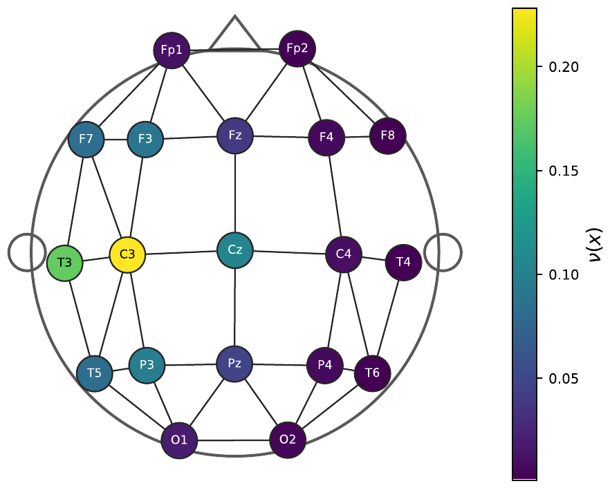
Social, transportation, sensor, and neuronal networks all carry data on the vertices of a weighted graph; today’s data are probability measures on the vertices
There is no grid and no coordinates, only the edges: the geometry of the domain is the graph
The question: how do we average such measures, and decompose one into others, in a way that respects that geometry?
A synthetic measure on the standard 10-20 system graph
Shuman, Narang, Frossard, Ortega, Vandergheynst. “The emerging field of signal processing on graphs.” IEEE Signal Processing Magazine 30.3 (2013): 83–98.
Optimal Transport:
A Tool for Comparing Probability Distributions
Optimal Transport Defines a Metric on Probability Measures
Kantorovich Problem, Wasserstein Geometry
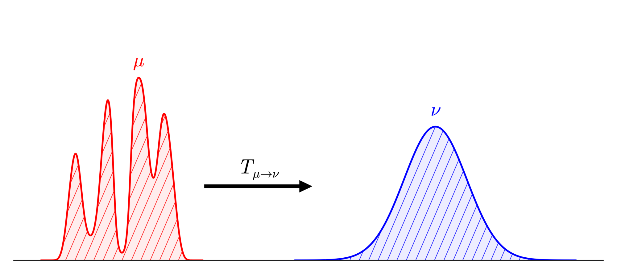
Let \(\mu, \nu \in \P(\R^d)\) be finite variance probability measures on \(\R^d\). Then the optimal transport cost, denoted by \(W_2\), between \(\mu\) and \(\nu\) is given by the following optimization problem:
This is a special case of the Kantorovich problem (KP), but for historical reasons the distance between measures defined by this problem is referred to as the \((L^2\)-)Wasserstein distance
Background on Optimal Transport
How does transport encode information about the underlying domain?
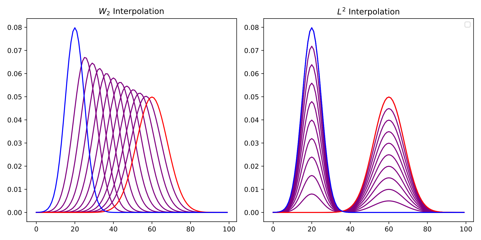
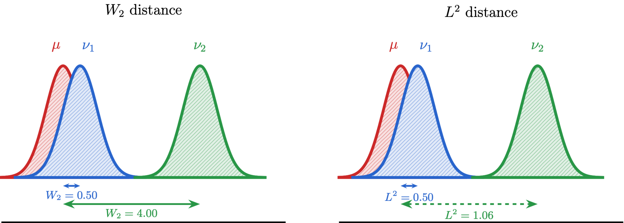
The \(W_2\) distance between two distributions tells us how expensive it is to move one to the other “physically”
This contrasts with, e.g., the \(L^2\) difference between the densities of two distributions, where mass “teleports”
Barycentric Coding Models
Averaging without linear structure
In \(\R^d\), a barycenter (AKA a weighted average) \(\bar x = \sum \lambda_i x_i\) of points \(\{x_i\}_{i=1}^p\) is also a minimizer for the function
\[ x \mapsto \sum_i \frac{\lambda_i}{2} \|x - x_i\|^2 \]
The latter is expressed through a squared distance, so it generalizes. With a transport distance it defines transport barycenters (Agueh–Carlier 2011 for \(W_2\)): for a dictionary \(\Refs = \{\nu_i\}_{i=1}^p\) and weights \(\lambda \in \Delta^{p-1}\), i.e. \(\lambda_i \ge 0\), \(\sum_i \lambda_i = 1\),
Two jobs: synthesis, given \(\Refs, \lambda\) compute \(\nu_\lambda\); analysis, given \(\nu_0\) and \(\Refs\) recover \(\lambda\)
Agueh, Carlier (2011); Werenski et al. (2022); in GW geometry, Chowdhury, Needham (2020) and Díaz Martín, Medri, Murphy (2025).
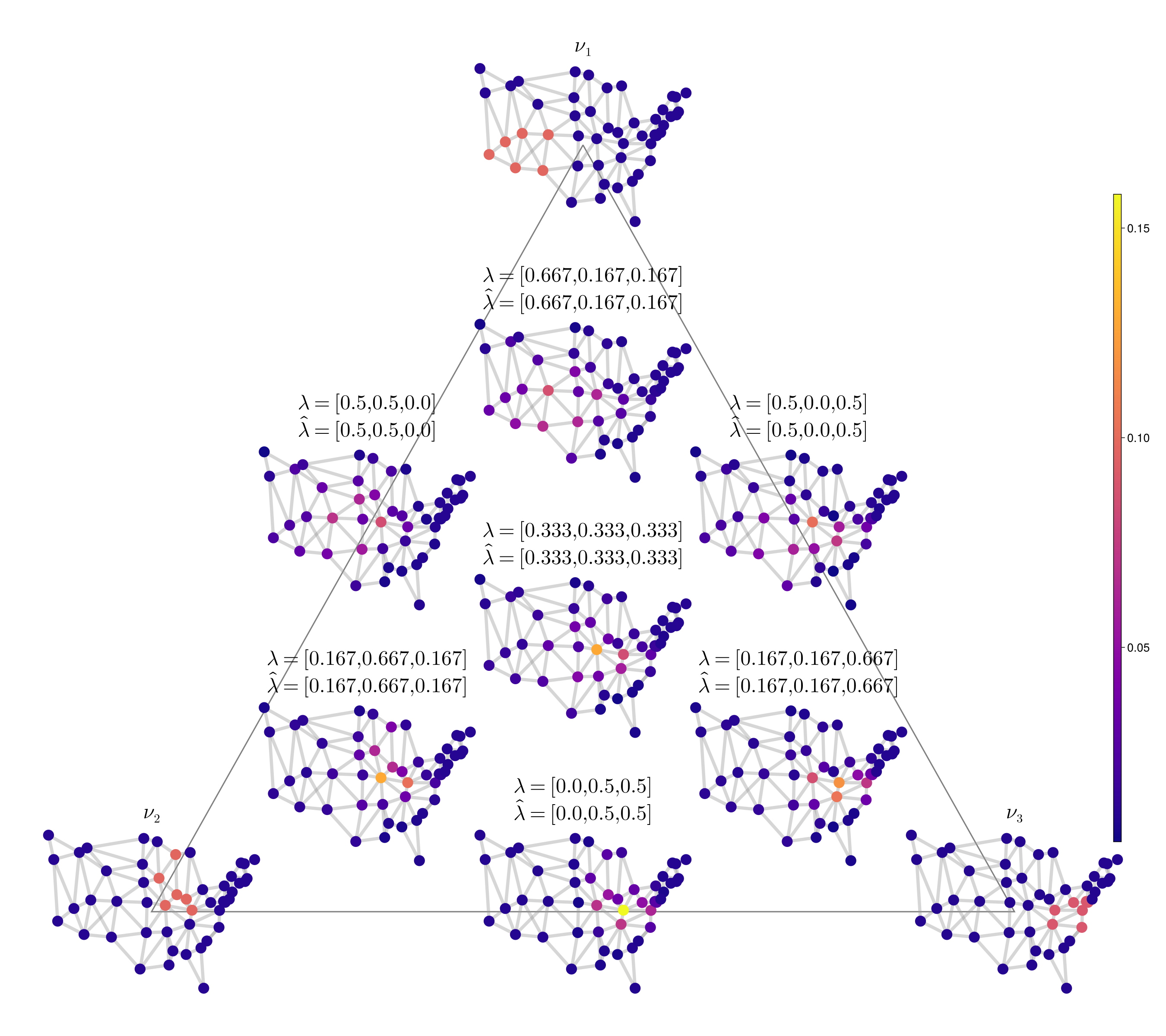
Example BCM
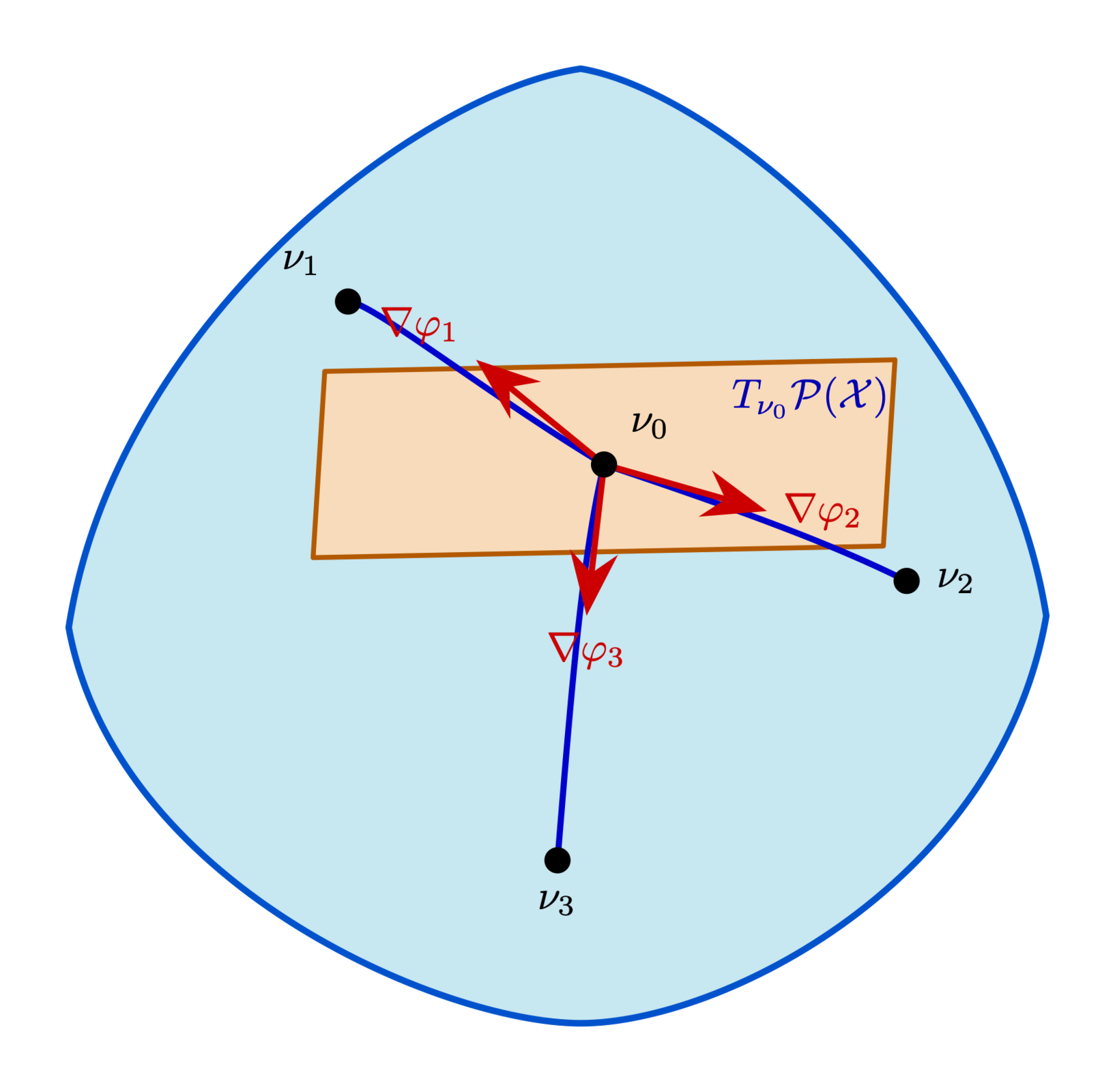
Vertices of the triangle: the dictionary atoms, three measures on the graph of the contiguous US states
Points inside: syntheses of the atoms
Each is annotated with its true \(\lambda\) and the \(\hat\lambda\) recovered by analysis: to \(4 \times 10^{-8}\) with Hamiltonian shooting; the paper’s Chambolle-Pock analysis of the same measures lands at \(10^{-2}\)–\(10^{-3}\)
Computed with the graph transport geometry of this talk; by the end you will know how
Why do this?
Applications of optimal transport on discrete domains & BCMs in general
Some things we can do with transport-based BCMs:
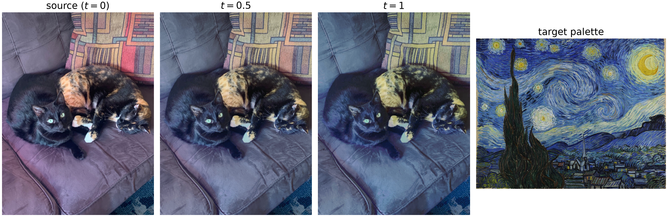
Automatic color grading of images, inferring reflectance functions & missing geometry (Bonneel et al. 2016, using entropic transport; next section)
Construct novel ways to study community segregation (Peng, Murphy 2025)
Sample efficient classification of point cloud data (Mallery, Murphy, Aeron 2025)
Color grading (after Bonneel et al.): quantize both images to 64 colors in CIELAB, so each image becomes a histogram, a probability measure on those 64 points; Bonneel et al. transport with the cost \(\|c_i - c_j\|^2\) on this fixed support. Here the 64 colors are joined into a 6-nearest-neighbour graph and the photo’s histogram moves along a graph-transport geodesic toward the painting’s: on a general graph the ground cost is replaced by transport along edges
Definitions
Graphs, Markov chains, and measures on them
A graph \(\X = (V, E)\), simple and connected, with symmetric edge weights \(\omega : E \to \R^+\) (\(\omega \equiv 1\) if unspecified), represented by the transition kernel \(Q\) of its random walk and the steady state distribution \(\pi\):
A function \(\varphi\) on \(\X\) lives on the vertices, \(\varphi \in \R^{|V|}\); a vector field \(\Phi\) lives on the edges, \(\Phi \in \R^{|V| \times |V|}\)
Probability measures are densities with respect to \(\pi\):
a simplex; its interior is \(\{\nu > 0\}\), its boundary the measures that vanish somewhere
Why is transport on graphs a problem?
Degeneracy of the Classical Transport Geometry when \(|\Omega| < \infty\)
Exercise to the reader: Let \(\X_2 = \{a, b\}\) be the two-point graph with a single edge. Characterize every coupling for a fixed pair of measures \(\nu_\alpha, \nu_\beta \in \P(\X_2)\) and solve KP explicitly
Conclude that \(\left(\P(\X_2), W_2\right) \simeq \left([0,1], \sqrt{|x-y|}\right)\)
Further conclude that if \(\nu(t) : [0,1] \to \P(\X_2)\) is a geodesic curve then it is constant! So you can’t even define a shortest-path between two measures on a two point graph.
Moral of the story: transport on a discrete space breaks if we come at it from the POV of coupled probability measures / KP
Two Ways Out
What do we do computationally about the degenerate transport geometry?
The Kantorovich problem is degenerate on a graph, but it is a linear program on matrices, and the BCM only needs a distance and a way to minimize \(\J\)
Solution 1 (static): keep the Kantorovich problem. Regularize it so it stops being degenerate, and feed it a cost matrix built from the graph. Cheap, and the graph is seen only through pairwise distances
Solution 2 (dynamic): replace the Kantorovich problem by the fluid-mechanical picture of \(W_2\) (Benamou–Brenier, coming up): \(W_2\) as the least kinetic energy of a flow carrying one measure to the other. Kinetic energy and flows make sense on a graph, and they define a Riemannian metric on \(\P(\X)\) that lives on the edges; the price is solving differential equations on the graph instead of a linear program
Solution 1: Keep Kantorovich, Regularize
Entropic transport on a ground metric built from the graph
A “Static” Approach to Barycenters of Measures
Entropic regularization: four steps to a BCM on a graph
Cuturi 2013. Regularize the Kantorovich problem with an entropy term: strongly convex, and Sinkhorn’s algorithm computes transport costs at “lightspeed”
Benamou, Carlier, Cuturi, Nenna, Peyré. “Iterative Bregman projections for regularized transportation problems.” SIAM J. Sci. Comput. 37.2 (2015): A1111–A1138.
Solution 1 in Practice
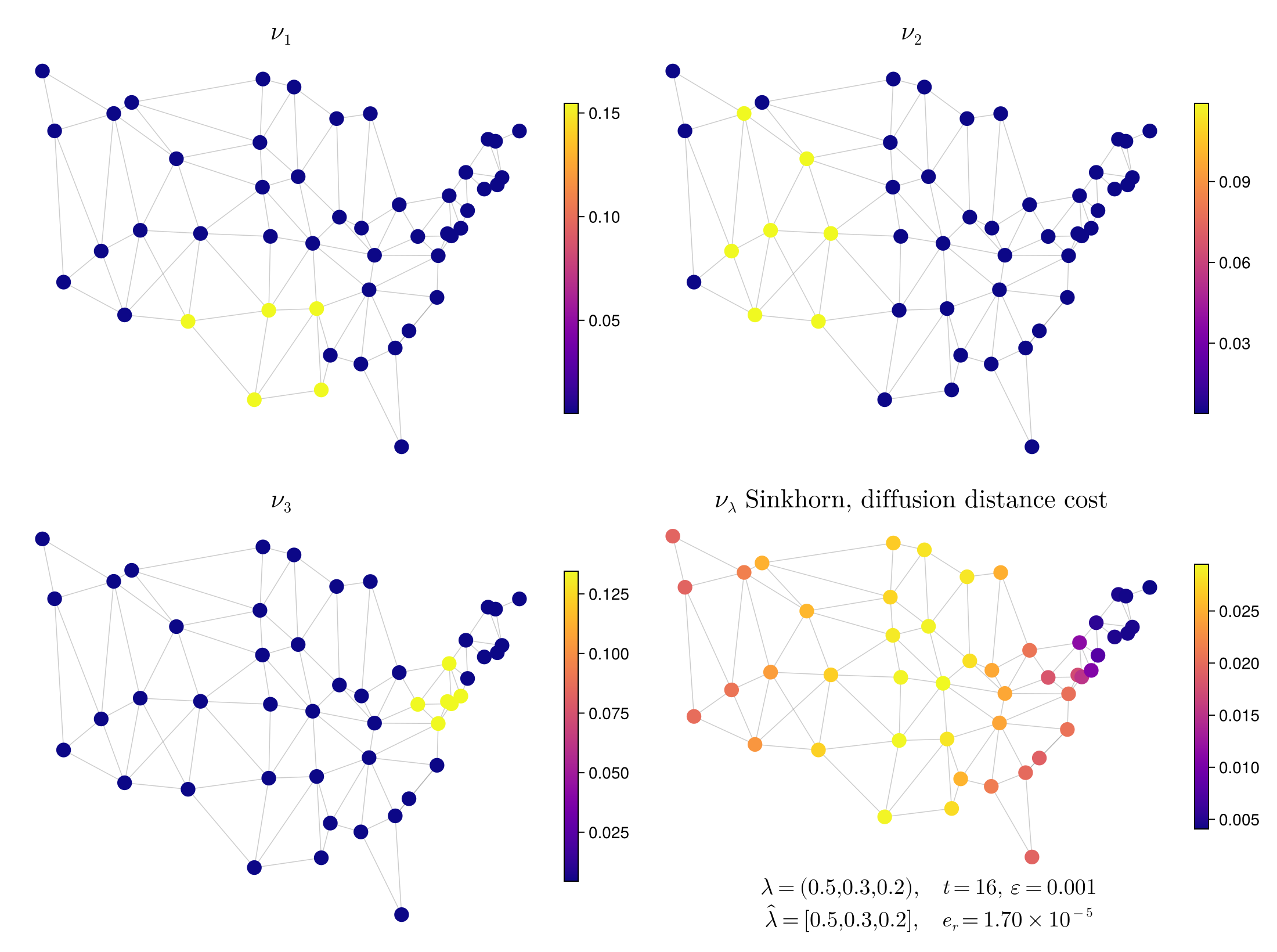
Regularized barycenters on the US states graph (G., Murphy, SampTA 2025)
The cost matrix comes from the graph: squared shortest-path distance, squared diffusion distance of the random walk at time \(t\), or a Fermat distance; Bonneel et al.’s fixed-support scheme does the rest
It works: synthesis and analysis both run, and the coordinates are recovered to a relative error of \(2 \times 10^{-5}\)
The drawback: a pairwise distance matrix does not encode edge connectivity, so the graph is seen only through distances; the entropy biases every output, and the geometry degenerates again as \(\varepsilon_{reg} \to 0\). What would a barycenter that sees the edges directly look like?
The SampTA experiment redone with the current code: squared diffusion-distance cost at \(t = 16\), \(\varepsilon_{reg} = 10^{-3}\), \(\lambda = (0.5, 0.3, 0.2)\); the recovered \(\hat\lambda\) and its relative error are under the panel
A second characterization of \(W_2\): it arises from a Riemannian structure on an “infinite-dimensional manifold” of densities, via the Benamou–Brenier formula
The infimum is taken over pairs \(\rho : [0,1] \times \R^d \to \R\), \(V : [0,1] \times \R^d \to \R^d\) which satisfy the continuity equation with temporal boundary conditions:
Benamou, Brenier. “A computational fluid mechanics solution to the Monge-Kantorovich mass transfer problem.” Numer. Math. 84.3 (2000): 375–393. The Riemannian reading is Otto’s: “The geometry of dissipative evolution equations: the porous medium equation.” Comm. PDE 26 (2001).
Continuity Equations on Graphs
The admissible mean
The construction that follows is due to Maas (2011), independently Mielke (2011) and Chow–Huang–Li–Zhou (2012); its Riemannian geometry is developed in Erbar–Maas (2012)
Plan: take the right-hand side of Benamou–Brenier as the definition of a distance on \(\P(\X)\). On a graph, \(\nabla\) and \(\nabla\cdot\) are easy (differences along edges, sums over neighbours); the trouble is the product \(\rho V\) in the continuity equation, a function on vertices times a vector field on edges
An admissible mean is a function \(\theta : \R^+ \times \R^+ \to \R^+\); it must be concave, lower semi-continuous, 1-homogeneous, symmetric, and \(C^2\) on \((0,\infty)^2\).
Read: the momentum \(m\) on each edge is charged against the mean \(\theta\) of the densities at its two ends, and \(\W\) is the least such kinetic energy along a path from \(\rho_A\) to \(\rho_B\). Benamou–Brenier, with \(\rho V\) replaced by \(\theta(\rho) \odot m\).
Maas, Jan. “Gradient flows of the entropy for finite Markov chains.” Journal of Functional Analysis 261.8 (2011): 2250–2292.
The \(\W\) Geometry
Riemannian Geometry Objects: Tangent Space & Metric Tensor
We’ll need to understand two things about the Riemannian geometry of \((\P(\X), \W)\): the metric tensor, and the exponential mapping
First, we need to say what the tangent space is, and how we can compute the inner product of two vectors at a point.
With \(\gamma_{\nu,m}\) the geodesic from \(\nu\) with initial velocity \(m \in T_\nu\P(\X)\):
\[ \exp_\nu(m) = \gamma_{\nu,m}(1), \qquad \exp_\nu^{-1}(\gamma_{\nu,m}(1)) = m, \qquad \exp_\nu : U \subset T_\nu \P(\X) \to \P(\X) \]
\(\exp_\nu^{-1}\) is single-valued on the ball of the injectivity radius; the radius of \((\P(\X), \W)\) is not known, and everything below assumes we stay inside it
The geodesic equation of \((\P(\X), \W)\) is explicit, as a Hamiltonian system in \((\rho, \varphi)\); that is the shooting section
An Implementation of a Barycentric Coding Model for Graphs
What existed, and what we add
Barycentric coding on graphs, before and after
Before. Barycentric synthesis and analysis for entropic \(W_2\) on a fixed support (Bonneel, Peyré, Cuturi 2016): Solution 1. For \(\W\), a convex program for one geodesic (Erbar et al. 2020), no barycenters
What we add. A BCM on \((\P(\X), \W)\) built from its Riemannian structure: intrinsic gradient descent for synthesis, a tangent-space Gram matrix for analysis, both driven by \(\exp_\nu\) and \(\exp_\nu^{-1}\)
Two ways to compute those maps. Erbar et al.’s space-time convex program (the paper): any pair of measures, sparsely supported ones included. Hamiltonian shooting on the geodesic equations (new): one to two orders of magnitude faster, interior measures only
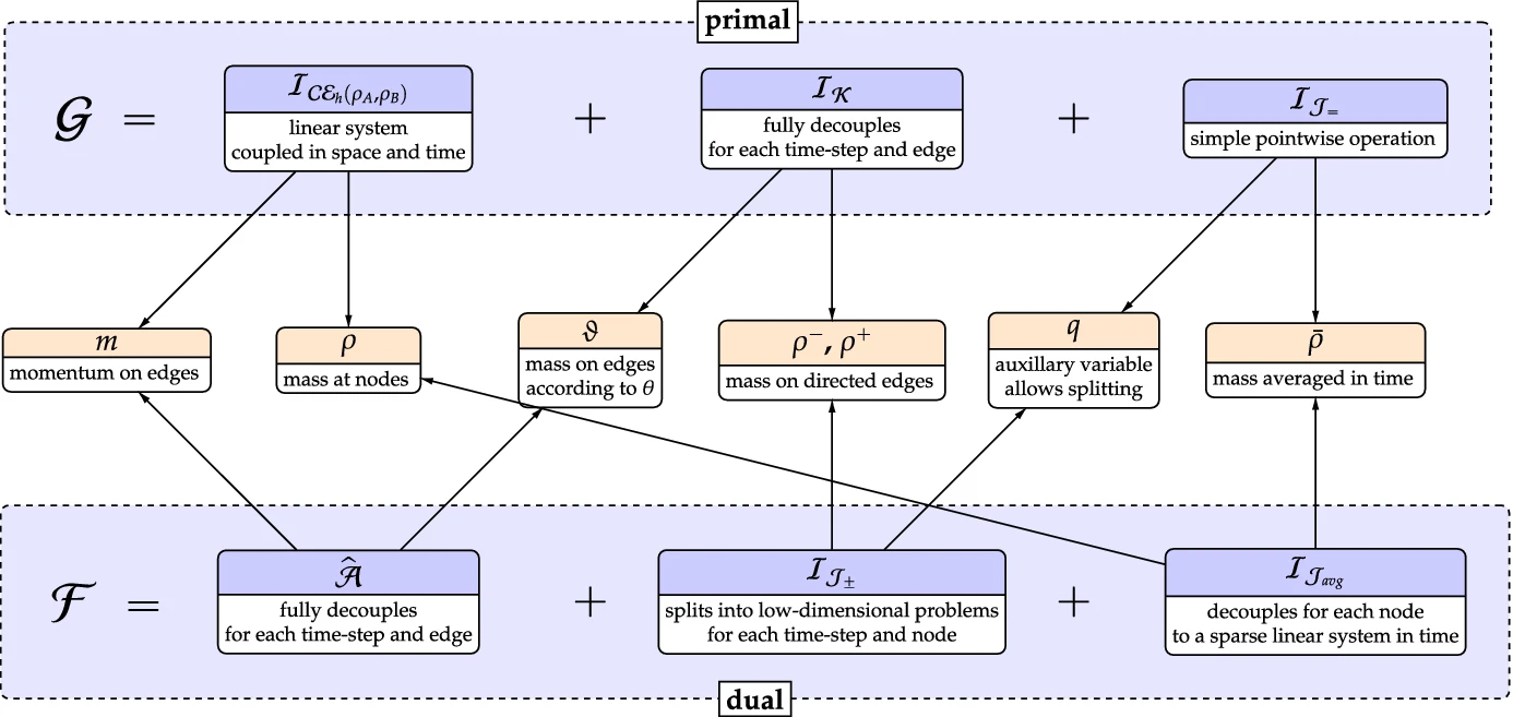
Chambolle-Pock solves problems in this form by operating on \(F^*, G\) one after the other, and the decoupling means that each sub-function can be addressed directly
This amounts to 4 linear algebra problems and two batches of geometric projections that are solved by Newton’s method
Decomposition of Erbar et al.’s algorithm
It’s simple, really.
Erbar, Matthias, et al. “Computation of optimal transport on discrete metric measure spaces.” Numerische Mathematik 144.1 (2020): 157–200.
Synthesis: minimizing \(\J\)
Getting back towards barycenters
Recall that the variance functional is expressed directly in terms of a metric!
Minimizers exist: \(\nu \mapsto \W^2(\nu_i, \nu)\) is convex along linear interpolations (Erbar–Maas 2012), so \(\J\) is convex and continuous on a compact convex set. Uniqueness, and convexity along geodesics, are open
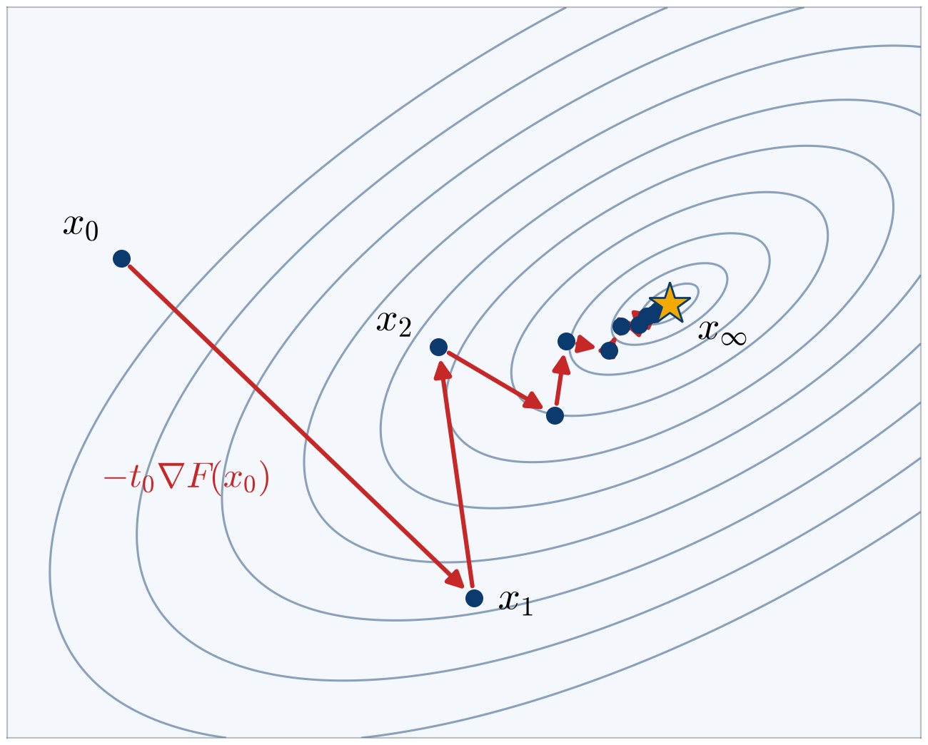
To find one, the oldest trick in the book: gradient descent. Find the direction in which \(\J\) decreases fastest and take a small step that way
Two problems: how do I know what direction to walk in, and how do I walk in it?
Erbar, Maas. “Ricci curvature of finite Markov chains via convexity of the entropy.” Arch. Ration. Mech. Anal. 206 (2012): 997–1038.
Synthesis Plan: Intrinsic Gradient Descent
When in Non-Euclidean spaces, do as the Non-Euclidean Optimizers Do
Gradient descent, \(x_{k+1} = x_k - t_k \nabla F(x_k)\): the same idea on \(\P(\X)\), with the intrinsic gradient of the Riemannian structure and steps along its geodesics
Absil, Mahony, Sepulchre. Optimization Algorithms on Matrix Manifolds. Princeton (2008). Huang, Absil, Gallivan. “ROPTLIB: an object-oriented C++ library for optimization on Riemannian manifolds.” ACM TOMS (2016).
Synthesis Plan: Reading the Two Maps
What \(\exp^{-1}\) and \(\exp\) mean on a graph, and how the paper approximated the step
Direction, \(\exp^{-1}_\nu(\nu_i)\): the initial momentum \(m_i(0)\) of the geodesic from \(\nu\) to \(\nu_i\): an edge field, the tangent vector from the geometry section, the first output of any geodesic solver. The descent direction for \(\J\) is \(m = \sum_i \lambda_i m_i(0)\)
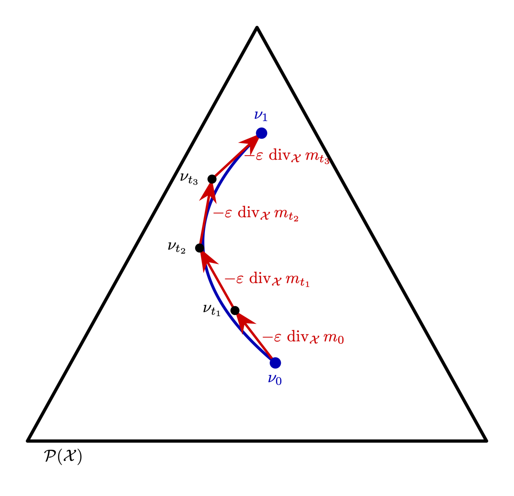
Step, \(\exp_\nu(\varepsilon m)\): the point at time \(\varepsilon\) on the geodesic launched from \(\nu\) with momentum \(m\). Geodesics solve the continuity equation, so near the launch point the step is one Euler step of it:
The heuristic: replace \(\exp\) by this first-order update: momenta from the geodesic solver (next slides), one sparse product for the step, mass conserved because \(\divX\) sums to zero
What it costs: the error is \(O(\varepsilon^2)\) per step, so \(\varepsilon\) must be small and the descent takes many steps, each needing \(p\) fresh geodesics
Synthesis Plan: Intrinsic Gradient Descent
When in Non-Euclidean spaces, do as the Non-Euclidean Optimizers Do
The update in Riemannian calculus: the direction is a sum of logarithmic maps, the step an exponential map. Those two maps are all the BCM needs. Last line: the paper’s Euler step from the previous slide; shooting computes both maps directly
Discretize space-time, then minimize the action as a convex program
Erbar et al. (2020): approximate \(\W\) by non-smooth convex optimization
Discretize \([0,1]\) into \(N\) steps, take a weak form of the CE, introduce slack variables to decouple the non-linear relations in the action, then minimize; the output is a discretized geodesic in the \(\W\) geometry
Works for any pair of measures, sparsely supported ones on the boundary included: the problem is convex and needs no interiority (remember this later)
Erbar, Matthias, et al. “Computation of optimal transport on discrete metric measure spaces.” Numerische Mathematik 144.1 (2020): 157–200.
Analysis Plan: Inverting The Exponential Map
Take it to the Tangent Space
To analyze a measure \(\nu_0\) against references \(\Refs = \{\nu_i\}_{i=1}^p\), we use a theorem of Werenski et al.
Theorem (Werenski, Murphy, Aeron et al. 2022, for \(W_2\) on \(\R^d\)). Let \(T_i\) be the optimal transport map from \(\nu_0\) to \(\nu_i\) and
Then \(\nu_0\) is the barycenter of \(\Refs\) with weights \(\lambda\) if and only if \(\displaystyle \min_{\lambda \in \Delta^{p-1}} \lambda^\top A \lambda = 0\), and the minimizer is \(\lambda\)
Why: the first-order condition for \(\J\) is \(\sum_i \lambda_i (T_i - \mathrm{Id}) = 0\), and \(T_i - \mathrm{Id} = \exp_{\nu_0}^{-1}(\nu_i)\) is a tangent vector, so \(\lambda^\top A \lambda = \|\sum_i \lambda_i \exp^{-1}_{\nu_0}(\nu_i)\|^2\)
On a graph: replace \(T_i - \mathrm{Id}\) by the log map and \(L^2(\nu_0)\) by the metric tensor at \(\nu_0\). Analysis is then \(p\) log maps, one \(p \times p\) Gram matrix, and a small quadratic program over the simplex
Werenski, Matthew, et al. “Measure estimation in the barycentric coding model.” International Conference on Machine Learning. PMLR, 2022.
Ambrosio, Luigi, Nicola Gigli, and Giuseppe Savaré. Gradient flows: in metric spaces and in the space of probability measures. Basel: Birkhäuser Basel, 2005.
Hyperparameters of the Algorithms
Our synthesis and analysis routines involve 4 hyperparameters:
\(\delta_g\) — convergence threshold for Chambolle-Pock, measures the weighted \(L^2\) norm difference between approximations of geodesics, default set at \(10^{-10}\)
\(N\) — number of steps per geodesic, defaults to 100 steps
\(\delta_b\) — convergence threshold for synthesis gradient descent, also an \(L^2\) norm measurement, default set at \(10^{-8}\)
\(\varepsilon\) — step size for gradient descent, default set at 1.0, dynamically shrinks if the step size takes the algorithm outside the admissible constraint set
N.B., each geodesic is expensive to compute, with complexity scaling quadratically in both \(N\) and \(|V|\)
Hamiltonian Shooting
Exponential and logarithmic maps without the space-time program
Where the time goes
The BCM only ever uses the start of a geodesic
Chambolle-Pock is a first-order method: reaching tolerances like \(\delta_g = 10^{-10}\) takes \(10^4\)–\(10^5\) iterations, each with a global space-time elliptic solve, over \(O(N \cdot |E|)\) variables
But look at what synthesis and analysis actually consume:
Synthesis: \(\exp_{\nu_k}\), and the initial momenta \(m_i(0)\)
Analysis: the initial tangent vectors \(\exp^{-1}_{\nu_0}(\nu_i)\), to build the Gram matrix
A geodesic is determined by its initial point and velocity, and satisfies an ODE of dimension \(2n\), independent of any time grid \(N\)
Idea: solve the geodesic ODE directly. \(\exp\) becomes an initial value problem; \(\exp^{-1}\) becomes a boundary value problem, solved by shooting
Geodesics as a Hamiltonian System
Position: the measure \(\rho\). Momentum: the potential \(\varphi\).
Stationarity of the action in \(m\) puts optimal momenta in gradient form, \(m_t = \theta(\rho_t) \odot \nabla\varphi_t\): velocities live in the tangent space from before
Stationarity in \(\rho\) gives the second equation. Together:
First equation: the continuity equation. Second: a discrete Hamilton–Jacobi equation. On a graph this is the Wasserstein Hamiltonian flow of Chow–Li–Zhou, in the form written down by Cui–Liu–Zhou
Chow, Li, Zhou. “Wasserstein Hamiltonian flows.” J. Differential Equations 268.3 (2020): 1205–1219. Cui, Liu, Zhou. “What is a stochastic Hamiltonian process on finite graph? An optimal transport answer.” J. Differential Equations 305 (2021).
What the Hamiltonian buys us
Conservation laws, and the distance from initial data alone
\(H\) is conserved along geodesics: constant speed, and a free accuracy check on any integrator
Total mass is conserved: it is the conserved quantity of the gauge symmetry \(\varphi \mapsto \varphi + c\)
The metric speed is \(\|\dot\rho_t\|^2_\W = 2H\), so
Given \(\nu\) and a potential \(\varphi_0\) (or a momentum \(m_0\), converted by one weighted-Laplacian solve), integrate from \(\rho(0) = \nu\), \(\varphi(0) = \varphi_0\):
\[ \exp_\nu(\nabla\varphi_0) = \rho(1) \]
In our implementation: fixed-step RK4, 150 steps on \([0,1]\); \(H\) and total mass drift by \(\sim 10^{-12}\) relative over the unit horizon
Interior only. The right-hand side of the ODE involves \(\partial_1\theta(\rho(x), \rho(y))\), which blows up as \(\rho(x) \to 0\): shooting needs \(\rho > 0\) everywhere and does not apply to sparsely supported measures, where Chambolle-Pock still does. A step that would push some \(\rho(x)\) below a positivity floor is bisected (up to 4 times) before giving up
Replaces the first-order heuristic \(\nu + t \operatorname{div}_\X m(0)\) in the synthesis update with an exponential map
The Logarithmic Map
Shooting: aim, fire, correct
To compute \(\exp_\nu^{-1}(\mu)\), solve for the initial potential:
with \(\kappa(x,y) = Q(x,y)\pi(x)\) the symmetric edge weight: the graph Laplacian with edge weights \(\kappa \odot \theta(\nu)\)
Warm starts: in an outer loop, the previous \(\varphi_0\) is an excellent initial guess
Shooting for the geodesic BVP is classical in shape analysis: Klassen, Srivastava, Mio, Joshi, IEEE PAMI (2004). For Wasserstein–Hamiltonian systems: Cui, Dieci, Zhou, SIAM J. Sci. Comput. (2022).
Closing the Loop: the BCM by Shooting
The synthesis update from before, without the approximation
Synthesis. With \(\varphi_0^{(i)}\) the potential of \(\exp^{-1}_{\nu_k}(\nu_i)\):
Each iteration: \(p\) log maps, warm-started from the previous iterate, and one exp map. Halve \(h\) if the step hits the positivity floor or fails to decrease \(\J\); stop when the descent direction’s metric norm \(\sqrt{2H}\) is small
Analysis. Log-map the target to each reference, build \(A_{ij} = \langle \nabla\varphi_i, \theta(\nu) \odot \nabla\varphi_j \rangle_Q\), solve the same quadratic program over the simplex
Two different time grids. Shooting still integrates the geodesic ODE on a grid of \(K\) RK4 steps, but that grid discretizes an ODE: error \(O(K^{-4})\), refined at will without touching Newton. Chambolle-Pock’s \(N\) steps discretize the action being minimized: error \(O(1/N)\), and every variable scales with \(N\). So synthesis and analysis should use the same method
A Geodesic by Shooting
3×3 grid, the example from the package tutorial
6 Newton iterations; round trip \(\|\exp_{\rho_A}(\nabla\varphi_0) - \rho_B\| \approx 8 \times 10^{-12}\); relative drift in \(H\) along the path \(\approx 8 \times 10^{-13}\)
\(\W^2 = 4.774998\) by shooting vs. \(4.537\) and \(4.644\) from Chambolle-Pock at \(N = 20\) and \(40\), which approaches from below at rate \(O(1/N)\)
How fast?
Random interior endpoint pairs on grid graphs, 20 trials each
25 nodes, 40 edges
100 nodes, 180 edges
Shooting \(\exp^{-1}\): Newton iterations, cold / warm
3–4 / 2–3
3–4 / 3
Shooting \(\exp^{-1}\): time
92 ms
1.6 s
Chambolle-Pock (\(N = 32\), \(\delta_g = 10^{-8}\)): time
Median wall-clock per geodesic, one CPU thread, after JIT warm-up. Chambolle-Pock is slow, so it was run on only 5 of the 25-node pairs and 1 of the 100-node pairs. The \(\W^2\) gap is Chambolle-Pock’s \(O(1/N)\) discretization of the action; shooting’s only discretization error is the integrator’s, \(O(K^{-4})\).
Shooting is one to two orders of magnitude faster than Chambolle-Pock, and the speedup grows with problem size: 34× at 25 nodes, 391× at 100 nodes.
Two Discretizations of the Same Geodesic
What each method discretizes, and what that costs
Chambolle-Pock (the paper)
Hamiltonian shooting (new)
What is discretized
the action, on a space-time grid
the geodesic ODE, in time only
Unknowns
\(O(N\,|E|)\): a path \((\rho, m)\) on \(N\) time steps
\(n - 1\): the initial potential \(\varphi_0\)
Error
\(O(1/N)\) in the time steps (Γ-convergence)
\(O(K^{-4})\) in the RK4 steps, refined at will
Iteration
first order: \(10^4\)–\(10^5\) primal-dual steps to \(\delta_g = 10^{-10}\)
Newton: 3–4 steps cold, 2–3 warm, to \(10^{-12}\)
Output
the whole path; the first-interval momentum
\(\varphi_0\), hence \(\exp^{-1}\) and \(\W^2 = 2H\)
Admissible data
any pair of measures, boundary included
interior of the simplex only
Guarantee
global optimum of the discretized problem, with a duality gap
a stationary path; minimality certified against the convex program
Shooting is an Interior Method
What happens near the boundary of the simplex
\(\partial_1\theta(s,t) \to \infty\) as \(s \to 0\): like \(\tfrac12\sqrt{t/s}\) for the geometric mean, like \(t/(s\log^2(s/t))\) for the logarithmic mean. Either way \(H\) is not \(C^1\) up to the boundary
This is geometry: a solution either exists for all time or, at some finite \(T\), some \(\rho(x) \to 0\) or \(\varphi \to \infty\) (Cui–Liu–Zhou 2021, Remark 3.3); geodesics can touch the boundary even between interior endpoints, and uniqueness can fail there (Gangbo–Li–Mou 2019)
In practice: mollify toward uniform, \(\nu_\varepsilon = (1-\varepsilon)\nu + \varepsilon\mathbb{1}\), shoot for decreasing \(\varepsilon\) (warm-started), extrapolate; for boundary-supported data, Chambolle-Pock remains the reference
Gangbo, Li, Mou. “Geodesics of minimal length in the set of probability measures on graphs.” ESAIM: COCV 25 (2019): 78. Cui, Liu, Zhou. “What is a stochastic Hamiltonian process on finite graph? An optimal transport answer.” J. Differential Equations 305 (2021).
Validating the Code with Numerical Experiments
Validation
How do we know if the thing actually works?
The code is validated by a suite of numerical experiments, looking at the following list of sanity checks:
Invariants of the Hamiltonian flow along every integrated geodesic: \(H\) and total mass conserved (relative drift \(\sim 10^{-12}\)), round trip \(\exp_\nu(\exp_\nu^{-1}\mu) = \mu\) to \(10^{-10}\), time-reversal symmetry, and \(\sqrt{2H}\) against the closed-form distance on the two-point graph
Agreement between independent solvers: do intrinsic descent with Chambolle-Pock geodesics and with Hamiltonian shooting land on the same barycenter?
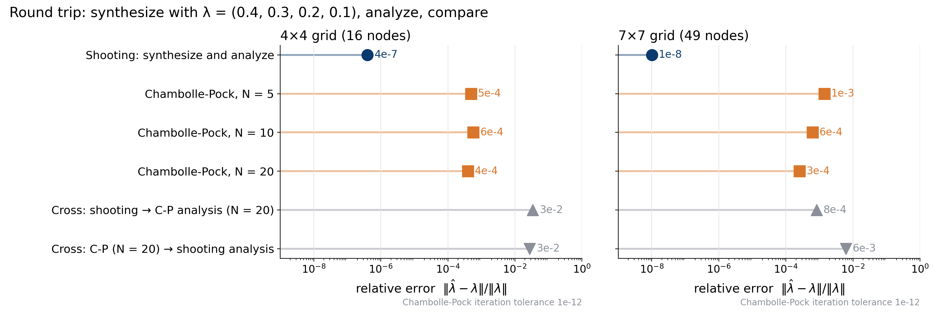
Round-trip consistency: synthesize with \(\lambda\), analyze to recover \(\hat\lambda\), check the relative error
Comparison with the popular alternative: entropically regularized transport on a cost matrix built from the graph
A Geodesic Three Ways
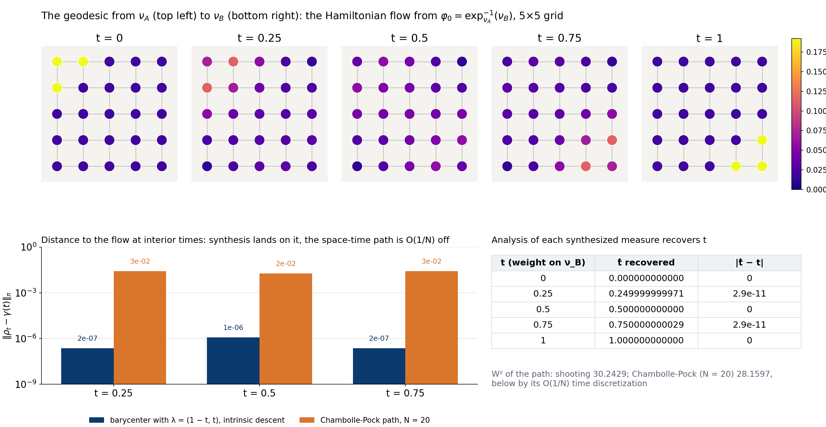
Synthesis with \(\lambda = (1-t, t)\), the geodesic equations, and Chambolle-Pock
Top: \(\gamma(t)\), the Hamiltonian flow from \(\varphi_0 = \exp^{-1}_{\nu_A}(\nu_B)\). Left: the barycenter with weights \((1-t, t)\) sits on \(\gamma\) to \(10^{-6}\); the Chambolle-Pock path at \(N = 20\) is \(10^{-2}\) off. Right: the coordinate recovered by analyzing the point at time \(t\) from each of the three sources
Two Solvers, One Barycenter
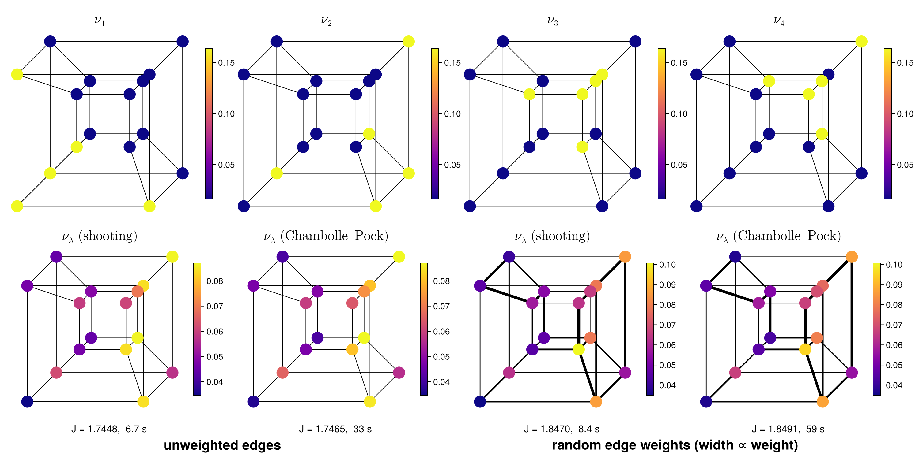
Intrinsic descent with Hamiltonian shooting vs. with Chambolle-Pock; same references, two edge weightings
Round trip: analyzing each shooting barycenter against its references recovers \(\lambda = (\tfrac14, \tfrac14, \tfrac14, \tfrac14)\) to \(\|\hat\lambda - \lambda\|_\infty = 9 \times 10^{-8}\) (unweighted) and \(1.5 \times 10^{-7}\) (weighted); the Chambolle-Pock barycenters, analyzed the same way, to \(5 \times 10^{-3}\)
Two Solvers, One Barycenter
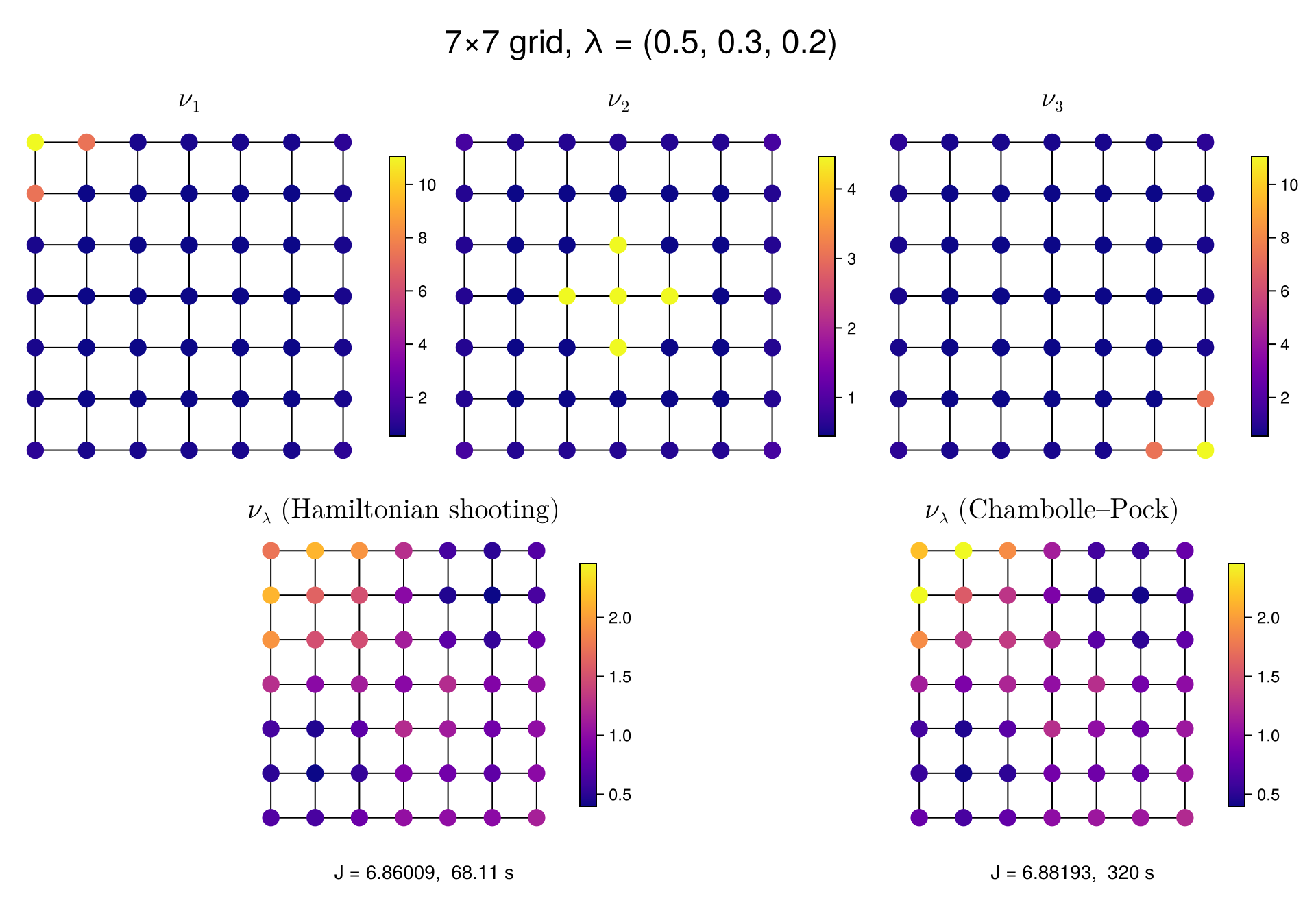
Intrinsic descent with Hamiltonian shooting vs. with Chambolle-Pock, 7×7 grid
Coordinate Recovery
Shooting recovers \(\lambda\) to \(10^{-7}\); Chambolle-Pock to \(10^{-3}\), bounded by its iteration tolerance
Solution 1 vs. Solution 2
Entropic transport on a graph metric against graph transport
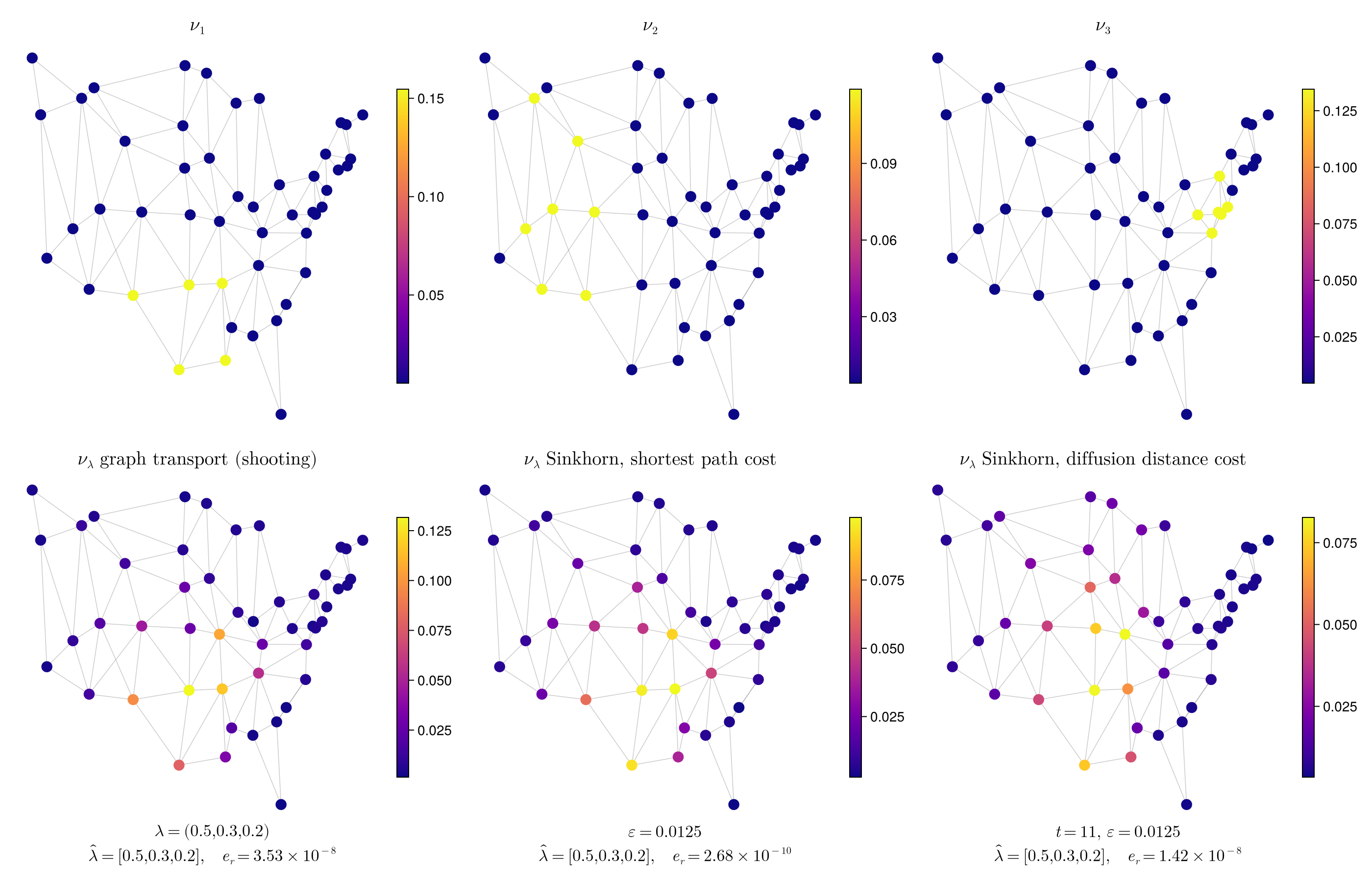
Back to the fork: Sinkhorn on a graph metric (Solution 1) against graph transport by shooting (Solution 2), same three references
Upside to entropic transport: very fast (about a second against a minute here); coordinate recovery is comparable, \(10^{-8}\) to \(10^{-10}\) for all three
Downsides: distance matrices don’t capture all connectivity information, entropy biases the output
Takeaway: only the graph transport barycenter operates directly on the graph structure
Summing Up
Takeaways on what we did
Barycenters need more than a metric: they need a geometry with geodesics, and the Kantorovich geometry on a graph has none (the two-point graph). The Benamou–Brenier picture survives the passage to a graph and gives the discrete transport metric \(\W\) of Maas, a Riemannian structure in which barycenters can be computed
Synthesis and analysis can both be handled by working within the Riemannian geometry of \((\P(\X), \W)\): intrinsic gradient descent for synthesis, the tangent-space Gram matrix of Werenski et al. for analysis. Both consume only \(\exp\) and \(\exp^{-1}\)
Computing those maps was the obstacle: the space-time convex program of Erbar et al. gives them at \(O(1/N)\) accuracy and \(O(N|E|)\) cost
New: Hamiltonian shooting computes \(\exp\) and \(\exp^{-1}\) directly from the geodesic ODE, accurate to fourth order in the integrator step (Runge–Kutta) rather than first order in a time grid, and one to two orders of magnitude faster on interior data
Impact of the Work
GraphTransportation.jl is:
The first publicly available implementation of Erbar et al.’s method, expanded to allow users to do novel signal processing work by exploring the geometry of a graph-based probability simplex via gradient descent
A significant step forward for the HILDA group and its long-running interest in data analysis problems set on graphs
About 4,000 lines of Julia library code, 250+ test assertions, and a suite of numerical validation experiments
Looking Ahead
Future directions and ideas to explore
Convergence theory for the descent. \(\J\) is convex along linear, probably not along geodesic, interpolation; in \(\R^d\) the same descent is saved by a Polyak–Łojasiewicz inequality. Does one hold on \((\P(\X), \W)\)?
Next: linearizing the BCM. Near a base measure \(\nu\), replace \(\exp^{-1}_\nu(\nu_i)\) by one weighted-Laplacian solve, \(L_\theta(\nu)\,\varphi_i = \pi \odot (\nu_i - \nu)\); on graphs, the discrete transport distance is locally a Laplacian quadratic form (Robertson, Wan, Cloninger 2024); this is linear optimal transport (cf. Wilson, Needham, Srivastava 2024)
Toward geodesic PCA on graphs: in the Wasserstein space over \(\R\), geodesic PCA becomes convex PCA in a linearized, tangent-space picture (Bigot, Gouet, Klein, López 2017). The linearized BCM supplies that picture for measures on graphs
References
My paper: G., Murphy. “Static and Dynamic Approaches to Computing Barycenters of Probability Measures on Graphs.” arXiv preprint arXiv:2603.26940 (2026).
Wilson, Needham, Srivastava. “Fused Gromov–Wasserstein variance decomposition with linear optimal transport.” arXiv:2411.10204 (2024).
Bauer, Mémoli, Needham, Nishino. “Metric geometry of Lebesgue, Wasserstein, and Gromov–Wasserstein spaces: submetries, curvature, and geodesics.” arXiv:2608.11680 (2026).
Maas. “Gradient flows of the entropy for finite Markov chains.” J. Funct. Anal. 261.8 (2011): 2250–2292.
Mielke. “A gradient structure for reaction–diffusion systems and for energy-drift-diffusion systems.” Nonlinearity 24.4 (2011): 1329–1346.
Chow, Huang, Li, Zhou. “Fokker–Planck equations for a free energy functional or Markov process on a graph.” Arch. Ration. Mech. Anal. 203 (2012): 969–1008.
Erbar, Maas. “Ricci curvature of finite Markov chains via convexity of the entropy.” Arch. Ration. Mech. Anal. 206 (2012): 997–1038.
Erbar, Rumpf, Schmitzer, Simon. “Computation of optimal transport on discrete metric measure spaces.” Numer. Math. 144.1 (2020): 157–200.
Gangbo, Li, Mou. “Geodesics of minimal length in the set of probability measures on graphs.” ESAIM: COCV 25 (2019): 78. Erbar, Maas, Wirth. “On the geometry of geodesics in discrete optimal transport.” Calc. Var. PDE 58 (2019): 19.
Afsari, Tron, Vidal. “On the convergence of gradient descent for finding the Riemannian center of mass.” SIAM J. Control Optim. 51.3 (2013): 2230–2260.
Cui, Liu, Zhou. “What is a stochastic Hamiltonian process on finite graph? An optimal transport answer.” J. Differential Equations 305 (2021): 428–457.
Cui, Liu, Zhou. “Wasserstein Hamiltonian flow with common noise on graph.” SIAM J. Appl. Math. 83.2 (2023): 484–509.
Liu, Wu, Ye, Zhou. “Parametrized Wasserstein Hamiltonian flow.” SIAM J. Numer. Anal. 63.1 (2025).
Zhou, Zuo, Liu, Li. “Accelerated Markov chain Monte Carlo algorithms on discrete states.” arXiv:2505.12599 (2025).